Driving piezo actuators with linear amplifiers
Piezo actuators are widely used in today's applications. They are available in all kinds of shapes and relatively cheap. Large forces can be produced at precise and small movements.
However, the capacitive character, the required high voltages and currents make the control of piezo actuators difficult. The solution to this problem is the use of power-operational amplifiers.
In this TOP Tech Talk we explain how to use them.
The piezo basics
Piezoelectricity means electricity as a result of pressure. A simple example is a gas lighter used to light your barbeque.For industrial use and especially in motion control, it is a bit more complicated:
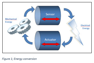
The piezoelectric effect is one of energy transduction. That is, a piezoelectric device can convert mechanical energy into electrical and vice versa. In converting energy from mechanical into electrical, the device behaves as a sensor. In converting energy from electrical into mechanical, the device behaves as an actuator (see figure 1, Energy conversion).
Let’s briefly look at the construction of a piezoelectric device. We start with bulk ceramic material with piezoelectric properties. That is, a crystalline structure that creates an electric field in response to mechanical forces or will expand or contract in the presence of an electric field.
Now, in order to more easily control the electric field, we add electrodes. Remarkably, the common symbol for a piezo device looks a lot like two electrodes with a block in between (see figure 2, Construction piezoelectric device).
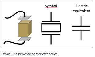
Electrically, two electrodes separated by a non-conducting – or dielectric – material is, by definition, a capacitor and as a first order approximation this is what we get with a piezo. As we will see a bit later, a piezo actuator does not behave as a pure capacitance, and this will have a direct effect on our control circuits and coaxing our desired motion out of these devices.
Piezo actuators
When we apply a voltage to the electrodes of our piezo device and create an electric field, a typical monolithic piezo crystal element will expand by only 0.01% of its overall length. So, to get an expansion of 0.1mm from a monolithic structure we need a device in the order of 1 meter in length.There are cost and manufacturability consequences to creating large monolithic piezoceramic structures, and as we increase the length of our device, the electrodes become further apart. The voltage required to maintain the electric field strength grows with the distance between electrodes. This can quickly become unpractical, and we are further limited by the maximum allowable voltage of the piezoceramic material.
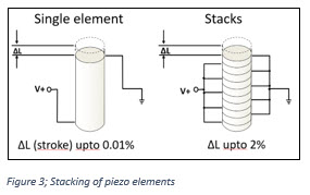
If, however, we interleave the electrodes and crystals, we can maintain a higher electric field with lower voltages. By keeping our fields stronger, a piezo stack can have stroke or displacement of up to 2% of its length. Even with a stacked configuration, the voltage requirements can range from 60V to several kilovolts.
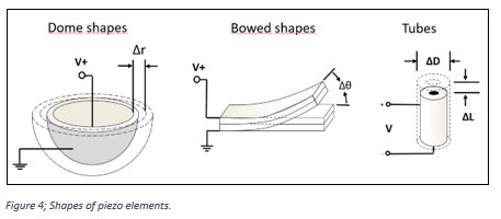
With these techniques different types of piezo actuators can be created, each with their individual shape:
Advantages and forces
Aside from all the physical implementations of the piezo actuators, there are other beneficial properties that make these actuators particularly useful:- Because the piezoelectric effect is electrostatic in nature, their use does not generate magnetic fields
- Nor are they influenced by magnetic fields.
- A piezo actuator holds its displacement with very high blocking force with no power dissipation.In fact, once the actuator is displaced, you could completely disconnect the electrodes and the piezo can maintain its displacement for weeks until leakage bleeds the charge from our capacitive structure.
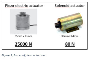
While their displacement, or stroke, may be small the forces generated by piezo actuators can be astounding, as shown in figure 5; on the left we see a piezo actuator and on the right side, we see an electromagnetic solenoid actuator of roughly comparable size. In fact, the solenoid is about twice the length of the piezo, but the force generated by this piezo actuator is over 300 times (!) that of the solenoid.
Because the piezoelectric effect is creating motion on the molecular level, there are really no moving parts in many piezo actuators. Consequently, they have very long lives with little or no wear.
This makes them low maintenance and clean and means they are compatible with vacuum environments.
They also have no mechanisms that bind or freeze at low temperatures. The piezo electric effect is useful even at temperatures as low as 4 Kelvin.
Creating and controlling movements
Now that we understand the structure and advantages of the piezo actuator, let’s look at the electronics control we need to provide to get the most out of these fantastic little machines.
We discussed earlier that the piezo element looks essentially capacitive. This is accurate, as the piezo element is nothing more than two electrodes separated by ceramic dielectric. The difficulty is that the dielectric in our capacitor is piezoceramic. This creates a mechanical system that will resonate at some frequency.
The electromechanical system of motion is modeled by the series LRC in parallel with our primary electrode and dielectric capacitor. The plot in figure 6 shows that the impedance rolls off nicely, like a capacitor should, until we reach resonance. Above resonance, the inductor of the electromechanical system is dominant and the LRC string becomes irrelevant.
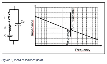
While piezo’ s may be used at resonance in free running, fixed frequency ultrasonic vibrators in some applications, most piezo actuators for arbitrary position or force control are used well below resonance. And the electromechanical effects do not affect our capacitive model.
The more relevant challenge with our piezoelectric capacitor model comes when we consider that capacitance is a function of the distance between electrodes. If our actuator is actuating, the distance between electrodes is not constant and we can get up to a 50% change in capacitance.
In the next steps we will explore actuator drive circuits and we will see that this variation in capacitance can have a significant impact on our choice of drive strategy.
The displacement or stroke of the piezoelectric device is proportional to the electric field we apply. The electric field is a function of our electrode voltage and the distance between them.
Because the distance between electrodes changes, the applied voltage is no longer a good way to predict or control the field. There are also some subtle mechanical phenomena that impact the relation of displacement and applied voltage including the nasty hysteresis effect that we see in the voltage vs displacement plot (see figure 7, Force proportional to the voltage).
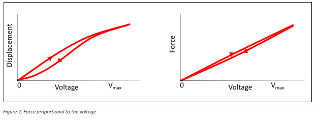
The good news, however, is that applied voltage does maintain a reasonable proportional relationship with the force generated by the actuator. A trace of hysteresis remains but is significantly reduced.
We can eliminate the distance between electrodes from our equations, by looking at charging the capacitor. We then find that charge on our capacitive structure holds a nice proportional relation with displacement over most of the range of motion of the actuator (see figure 8, Displacement proportional to charge).
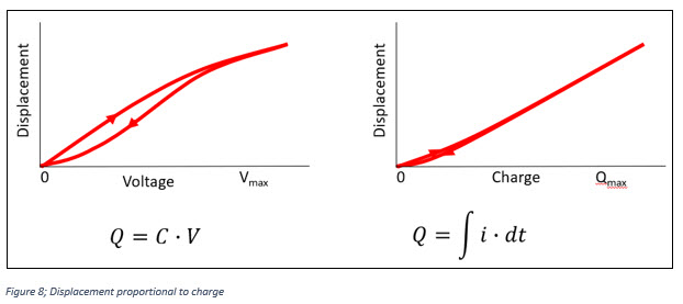
In fact, you may recall the earlier comment that a piezo actuator, once displaced, will hold its position even if the electrodes are disconnected. With disconnected electrodes, the charge will remain constant except for small leakage that one would find with any capacitor.
From what we just learned, our application requirements for force or displacement control demand that we have different strategies for our high voltage control electronics.
- Displacement of the actuator is proportional to charge
- Force generated by the actuator is proportional to applied voltage
Control electronics therefore depends on the application; Is it about displacement or strength?
Control electronics; choices and challenges
Because the voltages required for most piezo actuators are measured in hundreds of volts, drive electronics composed of discrete transistors can be very challenging. And pre-assembled solutions, including power supplies, housings, and support electronics can cost thousands of dollars each.
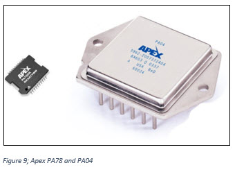
However, a design based around the high voltage op amp products from Apex Microtechnology can be cost effective and quick to market. The Apex op amp line includes a wide variety of features and performance. The products range from low-cost industrial integrated circuits like the PA78, a fast, high SMT IC, to military-grade hybrids, rated and tested for rugged, high temperature environments, such as the PA04.
The supply voltage of the Apex products ranges from 40V to 2500V and output current ranges from 10mA to 50A continuous. If these specs sound daunting, never fear. While they pack a lot of power, functionally these are op amps and designs based on them can be very straight forward.
Apex high voltage operational amplifiers make it simple to create drive system for precise force control. But there are a few challenges:
- Piezo actuator behaves like electrical capacitance
- Capacitive loads tend to destabilize a controlling circuit
- High speeds cause high currents
- Reactive loading of amplifier leads to additional power losses
- Piezo actuators can work as generators
Stability
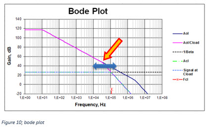
Together with the output resistance of the amplifier, the capacitive load causes an extra 'pole' in the so-called 'Bode plot' (figure 10, Bode Plot).
In some applications, the capacitive load is even dynamic! Examples are Industrial Inkjet printers, Analytical equipment, test & measurement equipment.
Dynamic capacitive load makes the resulting pole a 'moving target; stabilization of the amplifier has become more difficult.
Feedback factor
Control theory is applicable to closing the loop around a power op amp. The block diagram in the right of figure 11 consists of a circle with an X, which represents a voltage differencing circuit. The rectangle with Aol represents the amplifier open loop gain. The rectangle with the β represents the feedback network. The value of β is defined to be the fraction of the output voltage that is fed back to the input. Therefore, β can range from 0 (no feedback) to 1 (100% feedback).
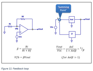
The term Aolβ that appears in the Vout/Vin equation above has been called loop gain because this can be thought of as a signal propagating around the loop that consists of the Aol and β networks. If Aolβ is large there is lots of feedback. If Aolβ is small there is not much feedback.
Rate of closure and instability
Aol is the amplifier’s open loop gain curve. 1/β is the closed loop AC small signal gain in which the amplifier is operating. The difference between the Aol curve and the 1/β curve is the loop gain. Loop gain is the amount of signal available to be used as feedback to reduce errors and non-linearities.
A first order check for stability is to ensure that when loop gain goes to zero, that is where the 1/β curve intersects the Aol curve, open loop phase shift must be less than 180° and, at the intersection of the 1/β curve and the Aol curve, the difference in the slopes of the two curves, or RATE OF CLOSURE, is less than or equal to 20 dB per decade. (See figure 12, Rate of closure).
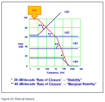
This is a powerful first check for stability. It is, however, not a complete check. For a complete check we will need to check the open loop phase shift of the amplifier throughout its loop gain bandwidth. A 40 dB per decade RATE-OF-CLOSURE indicates marginal stability with a high probability of destructive oscillations in your circuit.
Above examples indicate several different cases for both stable (20 dB per decade) and marginally stable (40 dB per decade) rates of closure.
Capacitive Load Implications
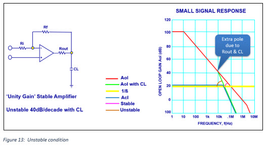
Even when using a unity gain stable amplifier, capacitive loads react with amplifier output impedance, which has the effect of introducing a second pole into the amplifier response which occurs above the unity gain crossover frequency.
If the amplifier is used at a low enough loop gain, this will result in the unstable condition shown in below graph. One simple solution is to increase the closed loop gain.
If it is necessary to use low gains with capacitive loads, or in the unlikely event they are a problem at higher gain, we describe 3 techniques that can help solve stability problems caused by capacitive loads:
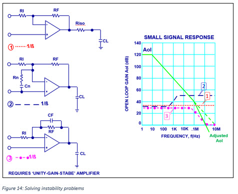
Method 1 uses a resistor in series with the amplifier output to isolate or cancel the capacitive load. Feedback should be taken directly from the amplifier's Aol output. In the graph, this has the effect of restoring the amplifier response to 20db/decade. This method has the advantage that with proper component selection, it can produce an overdamped or critically damped response to a square wave. The resistor is typically 1 to 10 ohms.
Method 2 uses ”noise gain compensation” to enhance stability. This method will work in virtually all cases. The idea is to set the ratio of RF/Rn for a gain high enough to insure crossing the Aol line at a stable point. The capacitor, Cn, is selected for a corner frequency one-tenth the Aol crossover frequency.
Method 3 uses a capacitor in the feedback path to cause a phase lead in the feedback which cancels the phase lag due to capacitive loading. This technique requires careful selection of capacitor value to ensure 1/b crosses the modified Aol before unity gain, unless a unity gain stable amplifier which has a good phase margin is used.
Power dissipation
Driving piezo actuators with Apex amplifiers is relative “easy”, it all comes down to Ohms law; V = I x R and P = V x I.
But we also need to consider that ![]() .
.
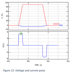
In below calculation example we can see what this means for the current (see Figure 15 for the wave forms):
Let’s assume:
.jpg)
- pulse amplitude=90V
- pulse rise-/fall time =2µs
Result:
![]()
The previously determined peak current is used to calculate the average power dissipation in the amplifier. As an example we take a circuit with the Apex amplifier MP108FD as in the figure below.
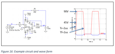
Assuming these pulse edges are linear, for our calculation we need to consider the center points of the rising and falling edges of the pulse and the voltage differences between the supply voltages (in this example +150V and -12V) and these center points.
First we calculate the power loss during the rising and falling edges. The center point of these edges is +45V and the voltage differences are Vd,r=150-45=105V en Vd,f=45- -12=57V
- The power loss of the rising edge is
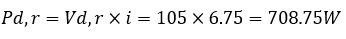
- The power loss of the falling edge is

Then we need to look at the duration of the falling and rising edges and determine the frequency of the pulse, which results in:
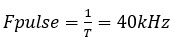
With these values we can then calculate the average power dissipation using
Quite hefty for a 150nF actuator! This means that good cooling is required.
Final precautions for your circuit
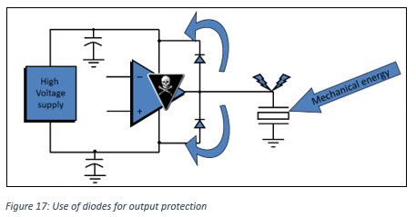
Piezo actuators can work as a generator when mechanically manipulated; this can create a lethal voltage kickback to the amplifier. Therefore, it is advised to use protection diodes as in below circuit example. These fast recovery diodes should have reverse recovery times of less than 100 nanoseconds.
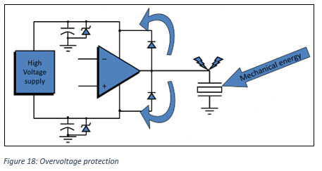
Also, we need to verify what the output impedance of the power supply is. This must look like a true low impedance source when current flows in the opposite direction from normal. Otherwise, the flyback energy, coupled back into the supply pin, will merely result in a voltage spike at the supply pin of the op amp. This would lead to an overvoltage condition and possibly destruction. These transients can be clamped using unidirectional transient voltage suppressor (TVS) diodes. Connect these devices as close as possible to the op amp’s supply pins.
All set?
We hope that with the above information you have learned more about piezo ceramic material, their use as an actuator and how to drive it safely with a linear amplifier. If you have any questions, please do not hesitate to contact us at [email protected].
References:
Presentation “Linear OpAmps for piezo’s” by Eric Boere, Apex Field Application Engineer
Apex application note “General Operating Considerations” AN01
Apex application note “Stability for Power Amplifiers” AN19
Apex application note "Driving Capacitive Loads" AN25
Apex application note "Driving Piezoelectric Actuators” AN44